A simple hill climber ↩
Before we get to talking about neural networks, let's start with something simpler. The very first homework assignment that I had in the course I mentioned was to construct a simple hill climber. The basic way these things work is simple:
You climb the hill.
But before you know what I mean by any of those words besides "the", we need to talk about terminology a bit and how a lot of this type of work is inspired by biology. As I mentioned before, the courses I was taking were all "evolutionary" CS courses. So, if we entertain the religion of modern day science for a bit, then we can happily state that over time, things evolve and become better due to random variations in genetics as well as the application of survival of the fittest.
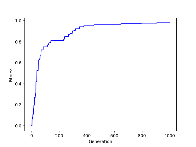
You can probably see where this is going. To "climb the hill" means that you get better over time, that whatever thing you're "evolving" does better and better. If you were to graph its progress, you'd see that however you're grading its "fitness", that it would increase. At the end of the day you'd have a graph with an upwards line that would eventually pitter patter out as no further gains were had. Something that looks like this:
There's a lot of ways you can implement this sort of thing. But the simplest is relying on cosmic rays and neutrinos. Which is to say, random pertubations of the "genome" you've created. We can also rely on computational eugenics! Which are not nearly as out of favor as human eugenics, so perhaps more like dog show breeding or horses? Basically, what I'm poorly trying to joke towards here is "breeding" of solutions.

But how does one "breed" computer programs? Well, there's actually a fair bit of interesting ways to do this. From genetic algorithms that have their operations and inputs in a tree that then gets swapped, mixed, and matched around to effectively construct mini programs; to large vector and matrix like "genomes" of data where some input has been converted into a representational structure with real values encoded into bits that can then be swapped around between parent genomes, much like the sort of things you study in high school biology with pea plants.
This has been a bit abstract so far, and "genome" might not mean anything to you yet. So, let's take a very simple example and show how we can "evolve" a genome through the power of a fitness function! As you may have guessed, a fitness function is, well, a way to measure how well something performed. This can be a simple function, like we're about to write, or it can be a full simulation of a bunch of events and then an evaluation of an end state or multiple states along the way. The fitness function is the guiding hand for our electronic life, and so it's important that we choose a good one when doing this sort of thing.
Here's a simple genome:
[ 0, 0, 0, 0, 0, 0, 0, 0 ]
These 0s could represent anything, but for now, let's just put aside any seeming usefulness, and instead come up with an arbitrary goal. We'll start simple, like trying to transform our list of 0's into a list of 1's.
Now, obviously, if our goal was to just make 0's into 1's, we'd just do something like
for element in list:
  element = 1
in our favorite language and be done with it. But, humor me, let's think about how we could "evolve" an initial vector, like the above 8 zeros in a list, into something that's closer to a bunch of ones. Our fitness function is fairly obvious here if you think about it for a moment:
def fitness_of_genome(genome):
  fitness = 0
  for gene in genome:
    fitness += gene
  return fitness / len(genome)
The average of all the elements in the list will be 0 when all elements are 0, and be closer to 1 the closer every element gets to becoming a 1.
>>> fitness_of_genome([0,0,0,0,0,0,0,0])
0.0
>>> fitness_of_genome([1,1,1,1,1,1,1,1])
1.0
And so we have our way to determine "survival of the fittest" in a mathematical way! Now, we just have to "evolve" the result. As I noted above, there's a lot of ways to do this, but we'll just roll with the simplest: genetic mutation. Supposedly, according to the theory of evolution, we can expect minor differences and variations over generations to result in people getting better and better at things by default. Or, in modern lingo, the people of today are just built different than yesterday.
So, let's define our evolution method:
def mutate_genome(genome, probability):
  child = genome.copy()
  for gene_index in range(0, len(child)):
    if random.random() < probability:
        child[gene_index] = random.random()
  return child;
As I said before, mutating the genome (or "perturbing" as my old homework says), in this case simply means flipping a coin. If we happen to fall within a certain range, then we update the gene. This doesn't strictly guarantee that the new child is more fit than its parent, in fact, it most likely means it's not! But in the game of evolution, it's all just praying to God that somehow you win the genetic lottery and come out with a thumb.
parent = [0,0,0,0,0,0,0,0]
child = mutate_genome(parent, 0.05)
print(parent) # [0, 0, 0, 0, 0, 0, 0, 0]
print(child)  # [0.3595610710945377, 0, 0, 0, 0, 0, 0, 0] <-- a thumb!
As far as telling whose got thumbs or not, we can use our fitness function to tell us that! And so, the code is as simple as you'd guess. If the child is more fit than the parent, than it gets to live on, knowing that its parent will die proud that the child has managed to live a better life than the parent ever knew.
def next_generation(parent):
  child = mutate_genome(parent, 0.05)
  parent_is_proud = fitness_of_genome(child) > fitness_of_genome(parent)
  if parent_is_proud:
    return child
  else:
    return parent
But, can something this simple really work? Let's find out if the idea of quantity will lead to quality is true by simulating it! Our fitness function will guide the evolution, acting as arbitrator for whomst will live, and who will be left to rot in the garbage collector:
parent = [0,0,0,0,0,0,0,0]
for generate in range(1, 1000):
  parent = next_generation(parent)

print(fitness_of_genome(parent))
print(parent)

# And a sample run:
.py
# 0.9722597951754005
# [
    0.9964594894202395,
    0.9636690556443653,
    0.9463922789805108,
    0.9717226186950639,
    0.9826137655478931,
    0.9650652439138652,
    0.9893626178869598,
    0.9627932913143068
]
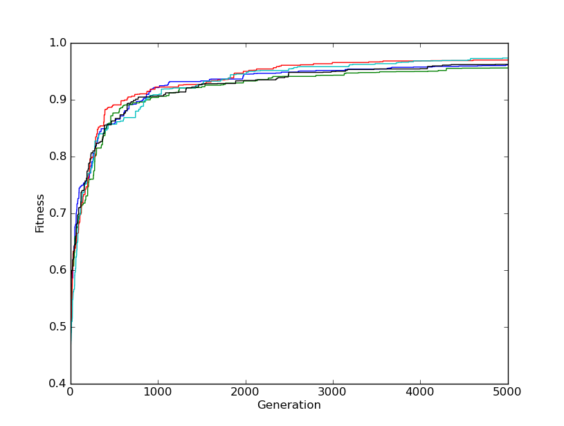
Surprised? You can run this code yourself and you'll likely see something similar, or you might witness evolutationary dead ends repeatedly. Just like life, there's a bit of randomness to it all. But this, in essence, is the hill climber. Because if we plot out the generational journey over time, then you can see how the fitness of the genomes "climb the hill":
It seems a bit silly perhaps to do it this way, and there are certainly other options available to us, but this was simply illustrative so that you've got a base idea about some of these concepts around how one "evolves" a solution. I don't want to cover it here, but look into genetic algorithms for some pretty cool stuff, I remember back in 2012 or so they were using these to come up with novel ways to structure satellites and such for durability. 5
Neural Networks ↩
Now that we've got an understanding of how a hill climber works, let's shift our focus back to what started this adventure. Neural networks are a bit more interesting than a single genome vector. They typically are set up to be connected and that gives them their intrinsic "net" like shape that gives them their name:
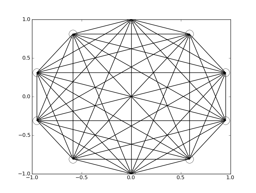
The above network is fully connected, meaning that each of its 10 nodes have a synapse, or connection, between every other node. In the above example the lines are just one thickness to show that a connection exists. However, the usual thing you'd see in a visualization like this wouldn't be a uniform line, but rather thickness or intensity of color being used to represent how strongly the given connection between two nodes in the net is.
In case it wasn't obvious by the usage of the word synapse and neural in the explanation so far: Neural Networks are modeled after the brain. Or at least, that's how the idea first came about, it, like most things powered by computers, quickly outgrew its biological counterpart, and new methods and techniques were layered on top of the original ideas. There's all sorts of really cool ideas around how to organize connections, what connects to what, if a network feeds signals only forward (feed-forward) or if it allows connections that send data backwards to prior nodes (back-progation and recurrent). There's a ton of really cool stuff to explore! But. Let's return to the simple for now and let me explain a bit more about these connections we've visualized so far.
In numerical form, the strength between two nodes is called the weight. And it can be used in all sorts of ways. The most common here though is as some form of multiplier on whatever signal passes through it. Say you had two nodes A and B. Both are connected to each other, but these connections are distinct. In other words, the connection from A to B is different than the connection from B to A. Specifically, the weight of the connection is different. For example:
| A | B | |
| A | 1.0 | 0.25 |
| B | 0.5 | 1.0 |
The connection to itself being strong doesn't have to be true but it does make my math easier in showing you the next important part here. The weights are used when calculating what the output of any given node is. Of course, to have an output somewhat implies that there is an input as well. So for the same of this example, let's assume that the input on the A node, and on the B node is just 1. And so, the output for the above two nodes would be calculation as:
| Node | Connections | Weighted calcuation | Weighted sum value |
|---|---|---|---|
| A | A → A + B → A | (1.0 * 1.0) + (1.0 * 0.5) | 1.5 |
| B | B → B + A → B | (1.0 * 1.0) + (1.0 * 0.25) | 1.25 |
The weighted sum of the connections coming into the node are a value that is typically than passed through what's called an "activation function". The result of which is the actual output of the node. There's a lot of ways to write up this function, such as doing something like:
if (weighted_sum > threshold_value):
   return 1.0
else:
    return 0.0
Which would be a simple step function. This sort of thing can be pretty useful when the output of your eventual network is intended to do things like classify data. Such as "yes, this picture is a cat". It's also handy for something like "turn on the rocket booster" or any sort of on-off behavior. The functions which we learned in my class way back when was the sigmoidal function:
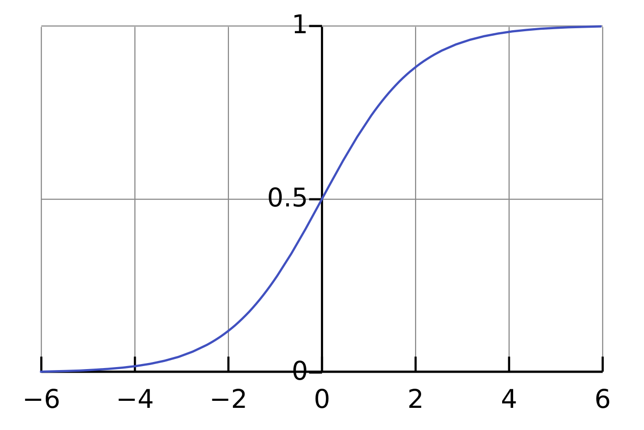
Which is useful since it normalizes its data to between 0 and 1 (or -1 and 1 in some cases) and helps to smooth things out a litle bit when you've got a lot of variation going on from whatever sorts of weights are going into your graph. According to Wikipedia it seems like there are other activation functions that perform better than this, but since that's what my homework assignments from over a decade ago used, I'll be using that to stick with what I know while I try to teach you all something.
Anyway. You've got a bunch of nodes and connections… How do you
actually make them do something for you? Well, we assumed there
was an input before, and there is! The important thing in a neural network,
as far as making it useful, is that there is an input and an output. Between
these two are any number of layers of neurons that bridge the gap,
and the result? A miserable pile of secrets Something known as a
multilayer perceptron. But enough talk, let's get to some code.
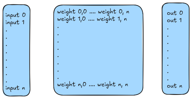
With our "genome" example, we used a simple vector of bits. With a dense
neural network that's fully connected between each layer, the choice between
an adjacency matrix or an adjacency list seems pretty obvious to me. But in
case you're unfamiliar, a 2D matrix with a value at (i,j) would
represent that there's a weight between the node i and node j. Or, if you're
thinking classical graphs, there's an edge between vertices i and j with
weight w. If we used an adjaceny list, we'd have a single list that holds
a reference to a linked list that begins with the first vertex i, and then
the connections from thereon out represent which edges connect back to j.
This is a sparser datastructure, but when we have to represent all edges anyway,
a matrix does this without as much overhead.
Also, it's going to make some math easier to understand if you're already familiar with linear algebra! Ahem. Code! Here's some simple code for creating our neural network layer:
def create_fully_connected_network_layer(number_of_neurons):
  rows = []
  for r in range(number_of_neurons):
    columns = [0] * number_of_neurons
    rows.append(columns)
  return rows


print(create_fully_connected_network_layer(4))
[
 [0, 0, 0, 0],
 [0, 0, 0, 0],
 [0, 0, 0, 0],
 [0, 0, 0, 0]
]
Now, how do we apply an "input" to this? Well. It's a matrix! And, if you're familiar with linear algebra, if you want to multiple an M by N matrix and get another matrix out, then we need to represent our input as a column of size N and then take the dot product. The dot product, convenientally, is the exact same formula that computes the weight sum. How fortuitious.
def input_vector(number_of_neurons):
  return [0] * number_of_neurons

def apply_input_to_layer(input_vector, layer_matrix):
  if len(layer_matrix) == 0:
    raise 'Matrix is empty'

  output_vector = []
  for i in range(len(input_vector)):
    input_value = input_vector[i]
    weighted_sum = 0
    synapses_to_vertix_i = layer_matrix[i]
    for incoming_edge_index in range(len(synapses_to_vertix_i)):
      weight = synapses_to_vertix_i[incoming_edge_index]
      weighted_sum += input_value * weight
    output_vector.append(weighted_sum)
  return output_vector
Note that we could use numpy for this. As there is a dot
and a bunch of other convenient matrix multiplication methods
through that library. But for learning purposes, let's stick to
writing it all out ourselves for now. Returning to our previous
example from before, we can confirm our logic is sound by repeating
the process from before:
number_of_neurons = 2
matrix = create_fully_connected_network_layer(number_of_neurons)
matrix[0][0] = 1 6
matrix[0][1] = 0.25
matrix[1][0] = 0.5
matrix[1][1] = 1.0
iv = input_vector(number_of_neurons)
iv[0] = 1.0
iv[1] = 1.0
ov = apply_input_to_layer(iv, matrix)
print(iv)
print(ov)
And this prints (unsurprisingly):
[1.0,  1.0]  # Our input vector
[1.25, 1.5]  # Our output vector
The same thing as we found when we did it by hand! Lovely. Now, these outputs from each node still need to be passed through an activation function to be translated into some real value that we care about. So let's define that:
def sigmoid(x, max_y, growth_rate, midpoint):
  return max_y / (1 + pow(math.e, - growth_rate * (x - midpoint) ) )

def logistic_function(x):
  return sigmoid(x, 1, 1, 0)
As noted before, we'll be using sigmoid curves for our activation function. The general formula is expressed above, and I pulled it right out of wikipedia. The second method is just a specific case of the function which is commonly called the "standard logistic function". We might as well do the standard thing for now, no reason to get fancy without a deep appreciation of what each type of formula does. Anyway, we're now able to express a single layered neural network:
This is useful in itself, but also, you can see how basic matrix multiplication
allows you to extend your "hidden layers" more deeply if you'd like. You can
have not just a single set of weights, but multiple, so long as the matrices
are all the same size and the math works out, you can do
IV * (M0 * M1 … *Mn) = OV
as much or as deep as you'd like. Though given that the product of all those
internal multiplications is going to be the same (because the multiplication
in these cases are associative), you can trivially say that all multi-layer perceptrons
can be reduced to just the one layer of weights + inputs. 7
Man, isn't linear algebra just a wonderfully fun thing?
Anyway. The last thing that we need to think about is how we "evolve" a network. Similar to the hill climbing example, we could do a simple mutation:
def perturb_layer(layer_matrix, with_probability):
  perturbed_layer = [0] * len(layer_matrix)

  for row in range(len(layer_matrix)):
    perturbed_layer[row] = [0] * len(layer_matrix[row])

    for col in range(len(layer_matrix[row])):
      if random.random() < with_probability:
        perturbed_layer[row][col] = random.random()
      else:
        perturbed_layer[row][col] = layer_matrix[row][col]
  return perturbed_layer
And this would be in line with the biological aspect of our simulation. We could also consider tossing out the idea that we should perfectly model nature, and instead use fancier methods such as backpropagation and gradient descent. This is only possible if we're doing supervised learning of our neural net though. Which means that we know the expected output, and want to help guide the way the weight values change accordingly.
For the purposes of keeping with our "evolutionary" theme, and because reading the wikipedia on backprogation is a mess of symbols and poor explanation, I'm going to skip over trying to explain that idea. My notes in the programs I have from my class are insufficient, and while I believe I have my notebooks in a box somewhere, I really don't want to dig them out to refresh on an idea that I'm not going to implement in code today.
Speaking of implementing, we could come up with some silly example like we did for the hill climber. But you've seen the computer make random mutations to a vector and "evolve" according to a fitness function already. I trust that you can generalize that idea to a full matrix of weights simply enough. So, let's skip that, and with our newfound foundational knowledge about very simple multi-layer perceptrons, let's move onto the fun and interesting part of this blog. 8
Predator and Prey ↩
Continuing our biological analogy. We're going to be taking survival of the fittest literally. Let's create a game of cat and mouse, where a cat's survival metric is if it can catch a mouse, and a mouse's survival metric is if it can avoid the cat.
If we were writing this up in a classical sense, we might look into Boids and put in some form of code that basically tells each creature to minimize or maximize the distance from the other. However, rather than us writing that code, we'll evolve it instead. The distance between the two is a good fitness function, so we can write that up easily if we know where our cat and mouse are sitting. We'll use a 2d world for simplicity:
def cat_fitness(cat_x, cat_y, mouse_x, mouse_y):
  """The larger this number is, the worst the cat did"""
  dx = math.fabs(cat_x - mouse_x)
  dy = math.fabs(cat_y - mouse_y)
  return dx + dy
And the mouse's fitness of course is the exact opposite of this! If we constrain our world to be within a specific size, then we can normalize the data a little bit and rather than having to remember to score one fitness metric as "biggest wins" and the other as "smallest wins"
def manhatten_distance(cat_x, cat_y, mouse_x, mouse_y):
  dx = math.fabs(cat_x - mouse_x)
  dy = math.fabs(cat_y - mouse_y)
  return dx + dy

def cat_fitness(cat_x, cat_y, mouse_x, mouse_y, world_x_limit, world_y_limit):
  cat_to_mouse_distance = manhatten_distance(cat_x, cat_y, mouse_x, mouse_y)
  max_distance = world_x_limit + world_y_limit
  return max_distance - cat_to_mouse_distance

def mouse_fitness(cat_x, cat_y, mouse_x, mouse_y):
  cat_to_mouse_distance = manhatten_distance(cat_x, cat_y, mouse_x, mouse_y)
  return cat_to_mouse_distance
Since we're in a 2d space, I'm using manhatten distance rather than linear distance that you'd normally think of. The math is a little easier and faster, and while nothing we're doing is hard here, it's nice to try to keep the parts that aren't a black box of neuratic magic to minimal complexity for illustration.
Speaking of illustration, let's draw our mouse and cat. Again, keeping things simple, let's just represent them as simple coloured dots:
world_x_limit = 2
world_y_limit = 2
cat_x = random.uniform(0, world_x_limit)
cat_y = random.uniform(0, world_y_limit)
mouse_x = random.uniform(0, world_x_limit)
mouse_y = random.uniform(0, world_y_limit)

cat_score = cat_fitness(cat_x, cat_y, mouse_x, mouse_y, world_x_limit, world_y_limit)
mouse_score = mouse_fitness(cat_x, cat_y, mouse_x, mouse_y)

# Let's have a plot that shows the cat and mouse, and their individual fitnesses
fig, (world_axes, fitness_axes) = plt.subplots(1, 2)

world_axes.set_title("World")
world_axes.set_xlim([0, world_x_limit])
world_axes.set_ylim([0, world_y_limit])
world_axes.scatter([cat_x], [cat_y], marker="o", c="#ff0000")
world_axes.scatter([mouse_x], [mouse_y], marker="o", c="#00ff00")

fitness_axes.set_title("Score")
fitness_axes.set_ylabel("Fitness")
fitness_axes.set_ylim([0, world_y_limit + world_x_limit])
fitness_axes.bar(['Cat', 'Mouse'], [cat_score, mouse_score], align="center")

plt.subplots_adjust(wspace=0.5)
plt.show()
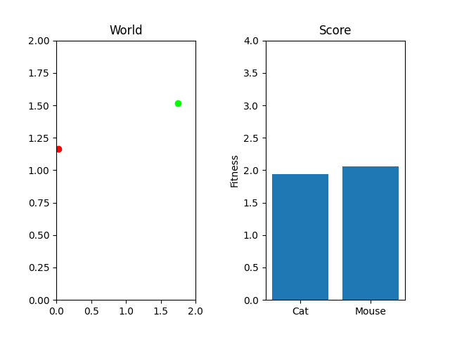
It's maybe not as exciting as doing something like using pygame to make a cute little cat chasing a mouse. But it will do the trick and we can visualize what happens over time once we put that code in. That said, the cat needs to chase the mouse. Starting them off randomly positioned and scoring the location doesn't actually represent our situation properly does it?
So, let's set up the "brains" of our friends. We'll use a multi-layer perceptron like I described in the last section, and we'll define our input layer to be the positions of our two creatures struggling to survive. The output of our system should map to what their new velocity vector is, and on every world-tick, we'll move the creatures positions. We could provide a continous scoring mechanism each tick, but that won't really let the neural net show off what it can do, so instead we'll limit the length of each simulation by a number of ticks, score it, then reset.
# Heavy perturbation at the start so we don't have all 0s
cat_brain = create_fully_connected_network_layer(4)
cat_brain = perturb_layer(cat_brain, 0.5)
mouse_brain = create_fully_connected_network_layer(4)
mouse_brain = perturb_layer(mouse_brain, 0.5)

# This is what "thinks" for the creatures.
def brain_tick():
  global cat_velocity, mouse_velocity

  cat_inputs = [cat_x, cat_y, mouse_x, mouse_y]
  pre_activated_output = apply_input_to_layer(cat_inputs, cat_brain)

  # -0.5 to give range of [-0.5, 0.5]
  dx_velocity = logistic_function(pre_activated_output[0]) - 0.5
  dy_velocity = logistic_function(pre_activated_output[1]) - 0.5
  cat_velocity[0] += dx_velocity
  cat_velocity[1] += dy_velocity

  mouse_inputs = [cat_x, cat_y, mouse_x, mouse_y]
  pre_activated_output = apply_input_to_layer(mouse_inputs, mouse_brain)

  dx_velocity = logistic_function(pre_activated_output[0]) - 0.5
  dy_velocity = logistic_function(pre_activated_output[1]) - 0.5
  mouse_velocity[0] += dx_velocity
  mouse_velocity[1] += dy_velocity

def clamp_to_world(x, y):
  new_x = max(0, min(world_x_limit, x))
  new_y = max(0, min(world_y_limit, y))
  return (new_x, new_y)

def world_tick():
  brain_tick()
  global cat_x, cat_y, mouse_x, mouse_y
  cat_x += cat_velocity[0]
  cat_y += cat_velocity[1]
  cat_x, cat_y = clamp_to_world(cat_x, cat_y)

  mouse_x += mouse_velocity[0]
  mouse_y += mouse_velocity[1]
  mouse_x, mouse_y = clamp_to_world(mouse_x, mouse_y)
Using globals like this is probably a little bit dodgy 9, but as you can see, we're really just doing exactly what I described before in the neural nework section. We've got inputs, the application to the network, and then taking the output through our "activation function" (in this case, the standard logistic function) and then each time the world ticks, we move our creatures based on their instincts.
The evolution of this cat and mouse game is just like the hillclimber we saw before, though I've got a bit more bookkeeping in order to generate some gifs for you.
generations = 10000
ticks_per_simulation = 25
cat_mutation_rate = 0.05
mouse_mutation_rate = 0.05
last_animation_frames = []
best_mouse_frames = []
best_cat_frames   = []

for i in range(generations):
  # The cat and mouse start somewhere random on the map
  start_locations()
  cat_velocity = [0, 0]
  mouse_velocity = [0, 0]
  last_animation_frames = []

  for _ in range(ticks_per_simulation):
    last_animation_frames.append(
        [cat_x, cat_y,
        mouse_x, mouse_y]
    )
    world_tick()

  cat_score = cat_fitness(cat_x, cat_y, mouse_x, mouse_y, world_x_limit, world_y_limit)
  cat_scores.append(cat_score)
  if cat_scores[i] < cat_scores[i + 1]:
    best_cat_frames = last_animation_frames
  else:
    cat_brain = perturb_layer(cat_brain, cat_mutation_rate)

  mouse_score = mouse_fitness(cat_x, cat_y, mouse_x, mouse_y)
  mouse_scores.append(mouse_score)
  if mouse_scores[i] < mouse_scores[i + 1]:
    best_mouse_frames = last_animation_frames
  else:
    mouse_brain = perturb_layer(mouse_brain, mouse_mutation_rate)
As you can see, I'm currently trying out a meager 10k generations with only 25 steps per simulation. This isn't really enough to actually "evolve" something, but it occasionally stumbles onto something that works. For example, here's the two best cat and mouse simulations from a random run:
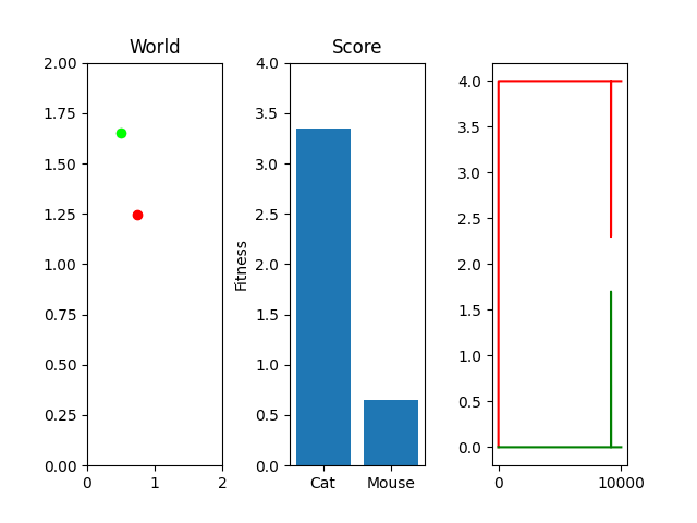
As you can see, the case where the mouse scored well, it actually had a death wish near the end. It starts getting curious about the cat, snifflying its way up the wall to its doom. Thankfully, the 25 steps its allowed to live ends and it enters the void of blissful unconsciousness before the cat chews its ears off. Playing God sure is horrific sometimes huh.

One thing you might notice that perhaps doesn't feel right at first is that our "hills" are no longer being climbed. There's random jagged jumps, peaks and valleys. For example, in this run, if you watch the best mouse run:
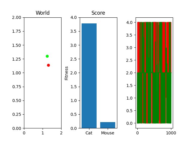
The mouse and cat happened to evolve in a way in which the cat is most definitely going to starve. However, the mouse did get to live! But look at the fitness values over generations on the righthand side. They're all over the place! What gives? You were promised rolling hills to climb, not jagged sharp edges! Well... we're evolving two competing functions here. When one gains, the other loses, and since they're very much dependent on each other, it's pretty tough to get something that shows that classic hill-like behavior.
There are ways you could try to deal with this of course. One could hold the cat steady in the middle, then train the mouse for a few generations, teaching it to stay away from the cat, then let the mouse train for a bit, repeat. However, the problem with this is that we risk overfitting to the training data. Holding the cat or mouse fixed might not teach it to chase after or run from the nemesis, but rather teach it to stay away from that one particular point in the graph. Then, when it comes to generalize, you'll end up with a creature that's paranoid and irrational about its world. Much like if you nearly choked on a piece of food once and then swore off eating it ever again because you happened to laugh during a meal.
Still. It's fun stuff I think. Here's the code that's plotting the above information and generating this gifs by the way:
def show_result_in_graph():
  # Let's have a plot that shows the cat and mouse, and their individual fitnesses
  fig, (world_axes, fitness_axes, fitness_over_time_axes) = plt.subplots(1, 3)

  world_axes.set_title("World")
  world_axes.set_xlim([0, world_x_limit])
  world_axes.set_ylim([0, world_y_limit])
  cat_scatter = world_axes.scatter([cat_x], [cat_y], marker="o", c="#ff0000")
  mouse_scatter = world_axes.scatter([mouse_x], [mouse_y], marker="o", c="#00ff00")

  fitness_axes.set_title("Score")
  fitness_axes.set_ylabel("Fitness")
  fitness_axes.set_ylim([0, world_y_limit + world_x_limit])
  barchart = fitness_axes.bar(['Cat', 'Mouse'], [cat_score, mouse_score], align="center")

  fitness_over_time_axes.plot(cat_scores, "-r", label="cat")
  fitness_over_time_axes.plot(mouse_scores, "-g", label="mouse")


  plt.subplots_adjust(wspace=0.5)
  frames = best_cat_frames + best_mouse_frames
  def animate(frame):
      cat_x, cat_y, mouse_x, mouse_y = frames[frame]

      # There is probably a better way to do this.
      cat_scatter.set_offsets([[cat_x, cat_y]])
      mouse_scatter.set_offsets([[mouse_x, mouse_y]])

      # Bar charts are weird.
      cat_score = cat_fitness(cat_x, cat_y, mouse_x, mouse_y, world_x_limit, world_y_limit)
      mouse_score = mouse_fitness(cat_x, cat_y, mouse_x, mouse_y)
      for i, bar in enumerate(barchart):
        bar.set_height([cat_score, mouse_score][i])

      return (cat_scatter, mouse_scatter, barchart)


  ani = animation.FuncAnimation(fig, animate, repeat=True, frames=len(frames), interval=200)
  plt.show()
  fig.savefig("cat_and_mouse_plot_sample1")
  writer = animation.PillowWriter(fps=15,
                                metadata=dict(artist='Me'),
                                bitrate=1800)
  ani.save('scatter.gif', writer=writer)
And for my last trick, let's do brain surgery. Remember that neat visualization I showed you at the start of the neural network section? The visualization of the weights of a fully connected 10 node graph? Let's see what our cat and mouse brains look like. We probably won't be able to make much sense of what each connection means, or derive any sort of meaningful function from inspecting the weights, but it's neat to see nonetheless:
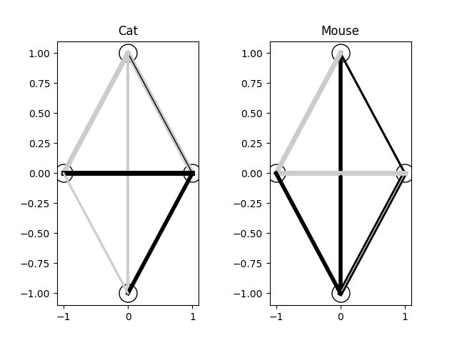
And the code to generate the visualization:
import matplotlib.pyplot as plt
import matplotlib.animation as animation
import math

CAT_BRAIN   = [...] # pull these from your simulation, a simple print(brain) will do!
MOUSE_BRAIN = [...]

def plot_synapse(axes, brain_matrix):
    nodes = len(brain_matrix)
    angle = 0.0
    angleUpdate = 2 * math.pi / nodes
    positions = []

    for i in range(nodes):
        x = math.sin(angle)
        y = math.cos(angle)
        angle = angle + angleUpdate
        positions.append([x,y])
        axes.plot(x, y,'ko',markerfacecolor=[1,1,1],markersize=18)

    for row in range(nodes):
        node_x, node_y = positions[row]

        for col in range(len(brain_matrix[row])):
            weight = brain_matrix[row][col]
            connected_x, connected_y = positions[col]

            line_width = int(10 * math.fabs(weight)) + 1
            color = [0,0,0]
            if weight > 0:
                color = [0.8, 0.8, 0.8]

            axes.plot([node_x, connected_x], [node_y, connected_y], color=color, linewidth = line_width)

fig, (cat_axes, mouse_axes) = plt.subplots(1, 2)
cat_axes.set_title("Cat")
mouse_axes.set_title("Mouse")

plot_synapse(cat_axes, CAT_BRAIN)
plot_synapse(mouse_axes, MOUSE_BRAIN)
plt.subplots_adjust(wspace=0.5)
plt.show()
There's a lot more you could do with this if you wanted to. For example, rather than random perturbation, you could crossbreed the "genes" of the node layers between parents. You could keep the top ten percent of each generation and then breed them. Heck, you could even breed the cat and mouse brains together since they're the same shape in this case (they don't have to be though! You could try to make the mouse "smarter" with more nodes!), as I said before, when we embrace the computing side of this and discard the biological origins, we can do all sorts of unethical strange ideas to see what results we can get.
In the class I took long ago we didn't actually do all of this in python. Some of it we did. But then the actual simulation code was done in C++ using the Open Dynamics Engine which supports rigid bodies. Our goal wasn't predator prey simulations 10 but rather getting a creature to learn how to walk. This was done by having the "brain" be created by the python program, then write the weights out to a file that the C++ program would read, run the simulation, then spit out the result into a fitness file for the python program to read and train more.
It was a bit wonky, as the presence of a fitness file that the C++ program had written out would trigger the python program's re-training, and similar, the creation of a weights file would result in the C++ program reading the data in. The file system as a sort of pseudo mutex led to some really annoying bugs when trying to leave the systems to train over long periods of time, which ultimately led me to just write the training code in C++ as well. But, since I wasn't trying to do a physics program today, I figured we'd stay in the easier to use Python world of matplotlib. 11
Anyway, I hope this was of interest. There are definitately better ways to train these types of things, but I'll just leave that as an exercise to the reader! That means you, Clonq. Let me know if this cleared anything up about how weights work in a neural net, if not and you're more confused than ever, well, you know where to find me. 12